Functions Forever
Use Excel functions to manipulate the data in the other sheets. Perform calculations, rearrange data, and create the custom format that you need.
This is nowhere near an exhaustive list of Excel functions. But, these are the ones that you'll most likely use as you get stared.
Simple Cell Reference
This is what you want to use when you know where (sheet and cell) the data you want is going to be located. For example, do you just want to pull the Issue Title out of the first column in the Dradis issues sheet? Perfect. Just create a function like:
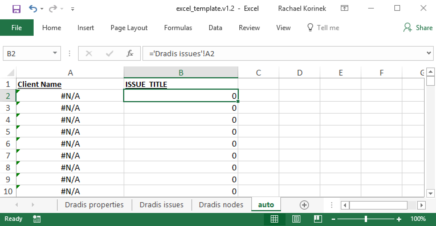
The syntax you want to use is: ='Sheet Name'!CELL
Example:
='Dradis issues'!A2
VLOOKUP
Use this function when you want to pull data from another column. For example, you can use VLOOKUP when you know the value in Column 1, but want to return the value in column 2:
| Column 1 | Column 2 |
|---|---|
| Known value | Value you want to grab |
This is especially useful for the Dradis properties sheet when you know that a value like dradis.client will be present somewhere in the first column, but the data you're after will be in the second column of the same row.
The example below will search for the dradis.client property in the Dradis properties sheet. If found, it will return the property value in Column 2 of the same row, not just return "dradis.client".
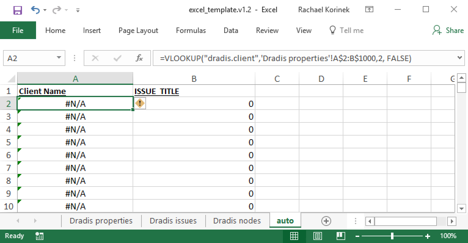
=VLOOKUP("dradis.client",'Dradis properties'!A$2:B$1000,2, FALSE)
Learn more about VLOOKUP on the Microsoft support site.
HLOOKUP
Use this function when you want to pull data from another row in your data. For example, you can use HLOOKUP when you know the value in the header row, but want to return the value in row 2 of the same column:
| Header | Known Value |
|---|---|
| Row 2 | Value you want to grab |
This is especially useful for the Dradis issues or Dradis nodes sheets where you know that the data you're after will be in a single column (e.g. Description):
=HLOOKUP("Description", 'Dradis issues'!A$1:Z$1000, Row(), FALSE)
Note the use of Row() above to reference the row index of the cell that contains the function. You can specify a numeric row (e.g. 2) instead. But, if you want to repeat this function for dozens or hundreds of rows in your template, you can quickly drag and replicate this function if you use Row().
Learn more about HLOOKUP on the Microsoft support site.
COUNTIF
Do you want a count instead of a value? Maybe you want to count the number of Critical Issues in your project so that you can populate a chart. Use COUNTIF to do this!
The example below will count the number of cells that have the value Critical in in cells B2 through B100 on the Dradis issues sheet. If none are found, the formula will display a zero.
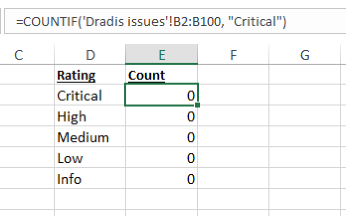
=COUNTIF('Dradis issues'!B2:B100, "Critical")
COUNTIF within a range
Do you need to count the number of values that occur within a range? Try a combination of functions like:
=COUNTIF('Dradis issues'!C2:C100,">=7.0")-COUNTIF('Dradis issues'!C2:C100,">8.9")
The function above counts the number of cells that have a value that is greater than or equal to 7.0. But, it also ignores all of the cells where the value is greater than 8.9. Together, this function will return a count of all of the cells that have a value between 7.0 and 8.9.
Learn more about COUNTIF on the Microsoft support site.
Charts and Graphs
First, make sure that you have the functions you need to populate the chart with the correct data! Then, COUNTIF is a great place to start!
Once you have the functions set up to calculate the data that you need in your chart, the rest is pretty simple. In the header of Excel, navigate to the Insert tab, then select the kind of chart you want (pie chart, bar chart, etc) from Charts.
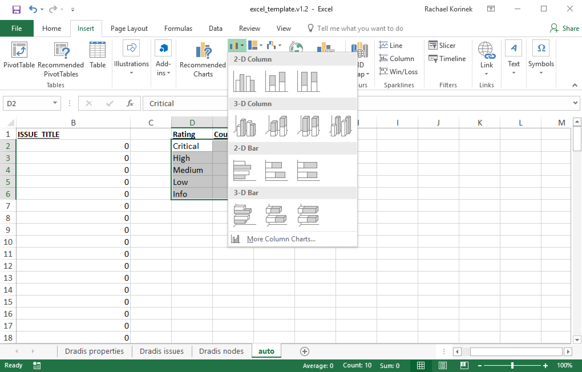
Now, the fun part! Play around with the way that the chart appears. Add background, add a title, add data labels, change the fill colors, do whatever else you want!
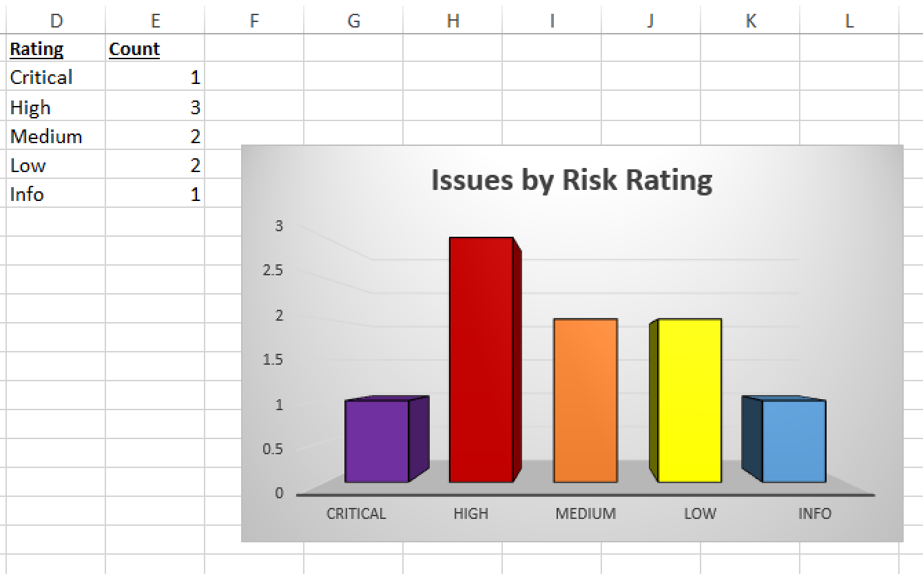
In the example below, we have a bar chart that displays the data from Columns D and E
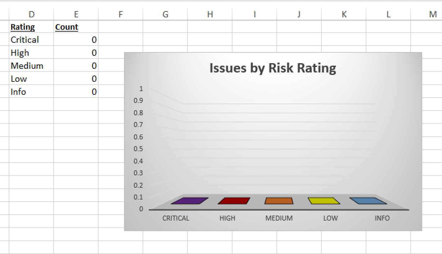
When we upload this Excel template into Dradis and Generate an Excel report, the chart will update with the real data from our project as shown below:
More and more complex
Start stacking your functions, add conditional logic, and get the results that you want! We'd recommend that you start small with a few simple functions, then build your formulas up one layer at a time.
You can find details and instructions for hundreds of formulas and functions on the Excel support website.
If you can dream it (and the data exists somewhere in your sheets), you can probably create a function to do it!
Overwhelmed? Contact our support team before you consider throwing your computer out a window. We're here to help!
Example: Return a Number (if present)
Do you need to return a numeric value (maybe for a CVSS score), but might have a non-numeric value in that cell (e.g. n/a)?
=IF(ISERROR(NUMBERVALUE('Dradis issues'!B2)),'Dradis issues'!B2,NUMBERVALUE('Dradis issues'!B2))
Let's break this down. In the case of this function, cell B2 on the Dradis issues sheet is going to contain a CVSS score that is either a numeric value, or n/a. So, we're starting with an IF statement. These statements are structured like:
=IF(logical_test, [value_if_true], [value_if_false])
In this situation:
- logical_test = ISERROR(NUMBERVALUE('Dradis issues'!B2))
- [value_if_true] = 'Dradis issues'!B2
- [value_if_false] = NUMBERVALUE('Dradis issues'!B2)
So, if the value from cell B2 on the Dradis issues sheet is not a number (e.g. if NUMBERVALUE throws an error), then we simply replace the cell with the value from cell B2 on the Dradis issues sheet. But, if the value is a number e.g. if NUMBERVALUE does not throw an error), we apply NUMBERVALUE to the value from cell B2 on the Dradis issues sheet to turn the text value into a number.
Example: Return blank if no value found
With a standard HLOOKUP function, the report will display 0 or #N/A if there is no corresponding value found in the referenced cell.
Instead of using the standard HLOOKUP function, you can nest the HLOOKUP inside of an IF statement so that you can display a blank cell if no value is found.
=IF(ISNONTEXT(HLOOKUP("Title", 'Dradis issues'!A$1:Z$1000, ROW(), FALSE)) = FALSE, HLOOKUP("Title", 'Dradis issues'!A$1:Z$1000, ROW(), FALSE), "")
The IF statement controls what is displayed in the cell. The logic test inside of the IF statement is ISNONTEXT(HLOOKUP("Title", 'Dradis issues'!A$1:Z$1000, ROW(), FALSE)) = FALSE. If the HLOOKUP returns a value that is text (e.g. ISNONTEXT = FALSE), the HLOOKUP value is displayed in the cell. Otherwise, a blank cell is displayed.
Return a Node property for an Affected host
Do you want more data on an affected host than just the Label field? If you want to pull the hostname, fqdn, or another Node property, you'll need to get a little creative:
=VLOOKUP(HLOOKUP("Label", 'Dradis issues'!A$1:Z$1000, ROW(), FALSE), 'Dradis nodes'!A$1:Z$1000, MATCH("fqdn", 'Dradis nodes'!A$1:Z$1,0), FALSE)
Let's break this function down from the inside out.
First, MATCH("fqdn", 'Dradis nodes'!A$1:Z$1,0) will return the index of the fqdn column on the Dradis nodes sheet.
Next level up, we're using a HLOOKUP function to return the Label associated with the specific instance of Evidence on the Dradis issues sheet: HLOOKUP("Label", 'Dradis issues'!A$1:Z$1000, ROW(), FALSE). Note the use of ROW() so that we're referencing the same row that the function lives in, allowing you to replicate this function for every row of data.
Now, at the top level, we're using a VLOOKUP function to search for the Evidence's Label within the Dradis nodes sheet, then returning the data from the fqdn column.
Next help article: Generate your Excel Report →